
Closed Loop Metrics for Earth Observation
Waymo Scaling, Waymo Insights

TLDR;
Just as GPT-style cross-entropy predicts language utility, Waymo shows motion cross-entropy tracks autonomous driving safety; we have yet to find the same appropriate objective for geospatial/EO.
Waymo shows their objective scales with compute budget in a similar fashion to LLMs.
We should think more carefully about deriving closed-loop-like metrics for earth observation to measure model utility, rather than model performance.
Autonomous Driving Scales
Waymo, the autonomous driving company whose burning cars became one of the enduring images of the Los Angeles anti-ICE protests, recently released a paper titled ‘Scaling Laws of Motion Forecasting and Planning: A Technical Report‘. In this report, the authors note that analagous to LLMs, the abilities of motion forecasting models also follow a power-law as a function of training compute.
The plot below shows this scaling for several different metrics:
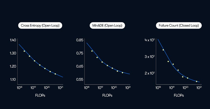
Cross-entropy (open loop): this is the training objective of the motion forecasting models. It is the likelihood that the model assigns to a given ground-truth trajectory/token sequence. Essentially: did the model think that what actually ended up happening was likely?
Minimum average displacement error (minADE): this measures the geometric accuracy of the best trajectory generated by the model relative to the ground truth. With this metric we ask the question: how close to the ground-truth can the model get if allowed to pick it’s best forecast.
Failure Count: the model is rolled out in a simulator and the number of failures in N scenarios is counted. Failures in this case could be collisions, going off-road, hard braking etc… here the key question is: is a given model safe if its own predictions feedback into decision making in a high-fidelity simulator.
Incredibly, we see that all three appear to improve with increasing compute budget, albeit with Failure Count appearing to flatten with larger compute budget. This tells us:
Next-motion-token prediction is a scaling-friendly objective
Lower loss appears to translate into safer simulated driving
Closed Loop Geospatial Metrics
Open- vs. closed-loop metrics are less common in the geospatial world; Waymo’s report illustrates them clearly. As you can see in the image above, only the Failure Count metric is ‘Closed Loop’: this means that the system is evaluated in scenarios where its actions directly influence the environment, and subsequently adjusts its behavior based on feedback received from the environment. This crucially evaluates an aspect of model performance that Open-loop metrics don’t by simulating driving ability in real-world driving conditions.
Why don’t we evaluate geospatial models in the same way? There’s been some discussion on whether benchmarks such as PANGAEA are useful, and my personal feeling is that benchmarks are the bare minimum, but ultimately we need some measure of the actually utility of these models, preferably in an operational setting. The tricky part in doing this if of course you need to connect to your end-user, and evaluate how changes in your model might affect them!
Of course, since we’re not automating an agent that interacts with the environment in geospatial (yet), the nature of the evaluation changes a little. However, below I provide some best attempts at imagining what some closed-loop/operational geospatial metrics could look like.
An Example: Flood Mapping
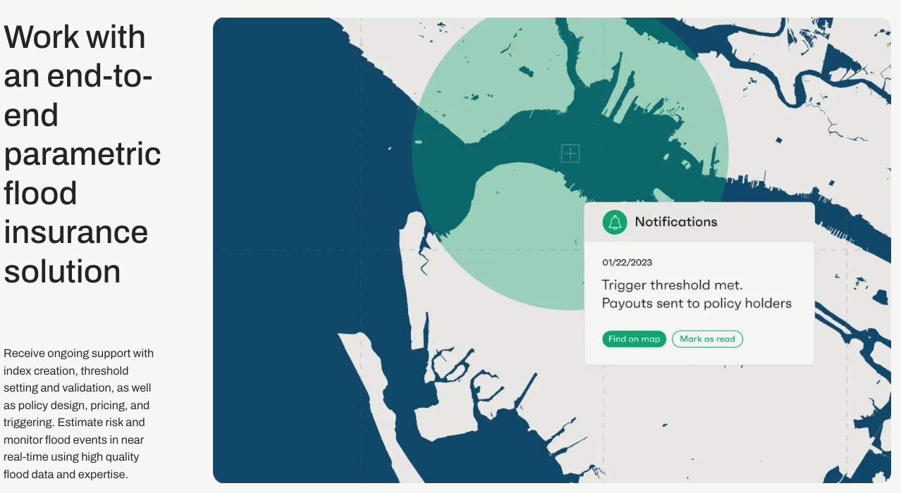
The Sen1Floods11 dataset is a part of the PANGAEA benchmarking suite, and is a “surface water data set including classified permanent water, flood water, and raw Sentinel-1 imagery.” A company in the insurance space may be interested in your fancy new model which blows every other model out of the water (no pun intended) on the Sen1Floods11 dataset. How can we move beyond just pixel-level skill in flood detection towards a more realistic and useful benchmark for such a business? By simulating how this model would actually be used in the real world.
For the sake of this thought experiment, let’s assume a parametric flood policy where the carrier agrees to terms such as: “if > X% of the insured polygon is inundated, as determined by the S1 flood model, then trigger a pay out”. This type of workflow is shown on the website of flood mapping company Floodbase:
A good closed-loop benchmark could be:
Replay an unseen year of Sentinel-1 acquisitions, task the model with emitting a trigger for each policy polygon when extent crosses >X%
Evaluate trigger F1 score for your polygons (did we fire on the right events/areas).
Evaluate basis-risk error (BRE) as defined by:
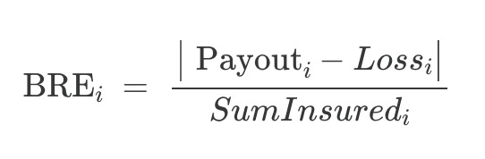
where Loss is the best available estimate for the monetary damage caused by the flood, Payout is what the model-drive trigger says the insurer must pay, and Sum Insured is the policy limit.
Now we get to see not only overall model performance at a pixel-level (IoU), but how it propagates through operational pipelines and ultimately affects customers. In effect we not only evaluate the ability of a given model to capture the signal of interest, but how model performance translates to decision performance and alignment with monetary loss. Thus when a new model is released, we can easily run it through our benchmark, and evaluate how IoU performance actually relates to our (fictional) bottom line.
Conclusion
There’s a lot of issues with the example I gave above: how can model developers access payout information, or insurance information? How can we accurately estimate the actually monetary value of the loss of a given property? These are questions that I do not have the answer to, but posing the question forces us to link model outputs to utility measured in dollars. A researcher I spoke to following the Geospatial Foundation Model diss piece told me that research in the field appears divorced from practitioners and end-users. They should rest assured that they are not alone in this: practitioners and companies themselves are often equally as separated from their clients and stakeholders.
Many organizations claim that the purpose of geospatial/earth observation is to drive decision making: in that case, why would we not also model that decision making process alongside the physical process we’re attempting to measure?
Thanks for the insight! It is certainly interesting to simulate impact-based downstream tasks for GeoAI.
But even for IoU, I'm curious about scaling laws in large-scale satellite imagery segmentation. Are there established rules/work for scaling architecture size and patch numbers to systematically improve segmentation performance?
Love the model utility concept. I am thinking it is important for usecases that target end user such as yield prediction. But this will mean every team/company will have their own benchmarking methodology as well results, so how can one tell which model is actually good in this case?