
Embedding Fields Forever
What Properties Should Geospatial Embeddings Have?

TLDR;
It is cool that people are releasing embeddings, kudos to the Deepmind/Google team!
Google’s Embedding Fields show large scale spatial variation that can be problematic for semantic search.
DuckDB is awesome, and can serve as a vector database.
Embeddings should be served at a scale that is larger than 10m pixels for ease of access.
Embeddings for retrieval should compress what is hard to join later (texture, specific land-use, shape), not what is trivial (elevation, lat/long, other raster dataset).
It’s important to do experiments with your embeddings: search and PCA are two easy ways to get a sense of the vibes.
As part of a recent project, I’ve been assembling various types of geospatial embeddings and testing out retrieval on them. This is all part of a bigger release of some open source tools that will hopefully enable you to do this type of analyses as well, which is coming soon!
Google Satellite Embeddings
One of the first embedding sets we turned to was the Google Satellite Embedding dataset: it’s a 64-dim embedding dataset that encodes ‘ temporal trajectories of surface conditions’ at each 10m pixel by ‘various Earth observation instruments and datasets’. It sounds like there’s a paper coming soon, but the only real information I could find was this conference poster, and this presentation. Between these two sources we can see that that various time-steps for various sources/sensors are encoded into a 64-dim latent space, and then decoded and used to reconstruct a set of amount of targets:
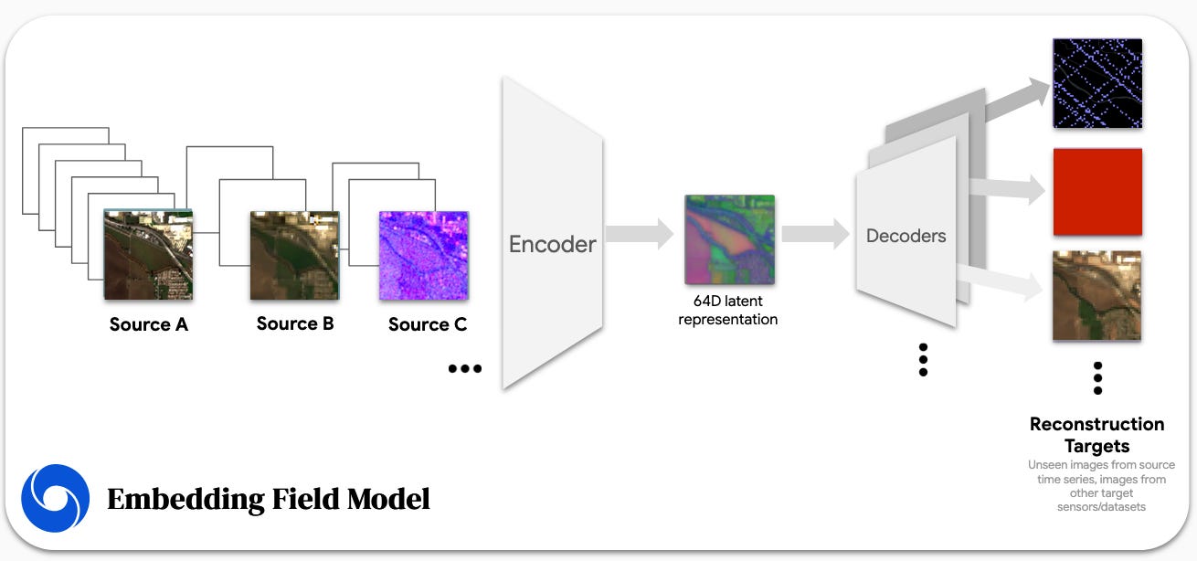
The poster gives us a little more clarity on exactly what these targets/reconstruction targets are:
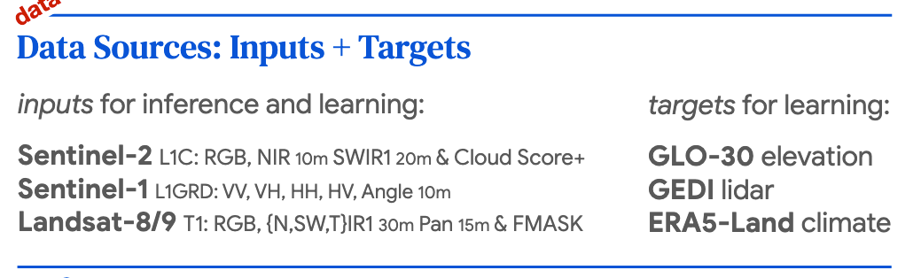
These are certainly interesting choices as targets for learning, and I’m not sure this is a particularly good idea, at least in the context of using embeddings for search or at large spatial scales. I’ll spend the rest of this post discussing why.
Pixels to (Geo)Parquet
The first step we need to take is aggregate these 10m pixels to larger tiles. This is because it is simply impractical to search over every single 10m pixel, and the Tobler’s law of geography tells us that things that are close together tend to be more similar anyway.
As a note to embedding providers: if you are considering pixel-level embeddings, you should also consider releasing an aggregated version at a coarser scale, this will help people explore you data more easily.
We can achieve this by first defining our tiles, uploading these geometries to Google Earth Engine (GEE) as GEE assets, and then simply performing reduceRegions over them. These operations allows us to export the the median for each embedding ‘channel’ over a tile (I chose 250m x 250m) as a geojson. We then end up with a 64-dim vector associated with each tile centroid, which we need to conver to geoparquet. In the case of the state of Alabama, this resulted in about 2.1 million embeddings.
As an alternative, you could export the embedding geotiffs from ee.ImageCollection("GOOGLE/SATELLITE_EMBEDDING/V1/ANNUAL", and perform the zonal stats yourself using rasterio/geopandas.
DuckDB
Once we have our embedding geoparquet files, containing tile centroid and a 64-dim embedding vector we can use duckdb to fulfill two purposes: it can act as a database such that we can easily retrieve batches of embeddings for the parquet file using SQL queries, but it also can act as a vector database for similarity searching thanks to the vss extension. Creating an Hierarchical Small Navigable Worlds (HSNW) index on top of your database is extremely easy just run:CREATE INDEX my_hnsw_cosine_index ON my_vector_table USING HNSW (vec) WITH (metric = 'cosine');
as you are creating your duckdb table.
This then allows you to use a 64-dim query vector to find ‘similar’ entries in your db. We ran into some interesting issues with scaling and performance that we will be writing up in some separate benchmarking posts, but this is the general gist of it!
Search
Now that we have a searchable vector db, we can simple choose a lat-lon and query Google’s Embedding Fields for similar points! In the video below, you can see me interactively querying the Embedding Fields for tiles that look ‘suburban’. We can see that it does a fairly good job with these! As we zoom out, we see detections concentrated on the periphery of major urban areas in Alabama. As we zoom into a different area, we see that the retrieved tiles have similiar ‘suburban’ characteristics to the query tiles.
This is a pretty neat way of getting a sense of any embedding datasets ‘vibes’ since you are able to tell how it does in terms of human-level semantics: you can search for any minority class of interest in your dataset, and see how well the embeddings have encoded that class as a ‘concept’. If the search results are similar tiles/things, then congratulations your model, and embeddings are good. At least when it comes to that particular search/class.
What Properties Should Embeddings Have?
As I started searching, I noticed some puzzling behavior: some searches seemed to work well (i.e the suburban neighborhood search from above). Others exhibited rather odd behavior, especially as I widened the scope of the search. For example: here I’m selecting a forest tile, and searching for the 25,000 closest neighbors in the embedding space. The search results show a very interesting spatial pattern!
In fact, I can reproduce the complement of this pattern, simply by seeding my search with a forest tile further south:
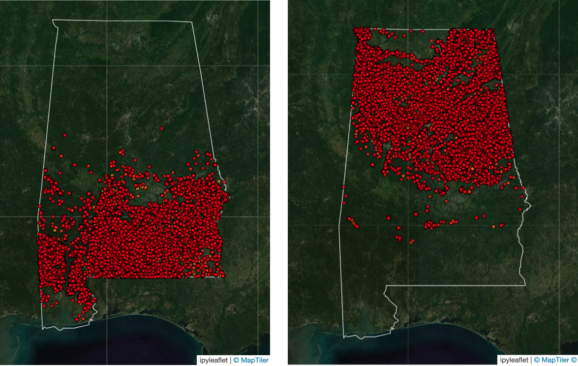
Interesting! I would expect these tiles to be somewhat semantically similar in any meaningful embedding space. I would also not expect to see this sort of dramatic geographic pattern, unless there was some underlying physical phenomena occurring driving changes in the satellite observations that constitute the embeddings.
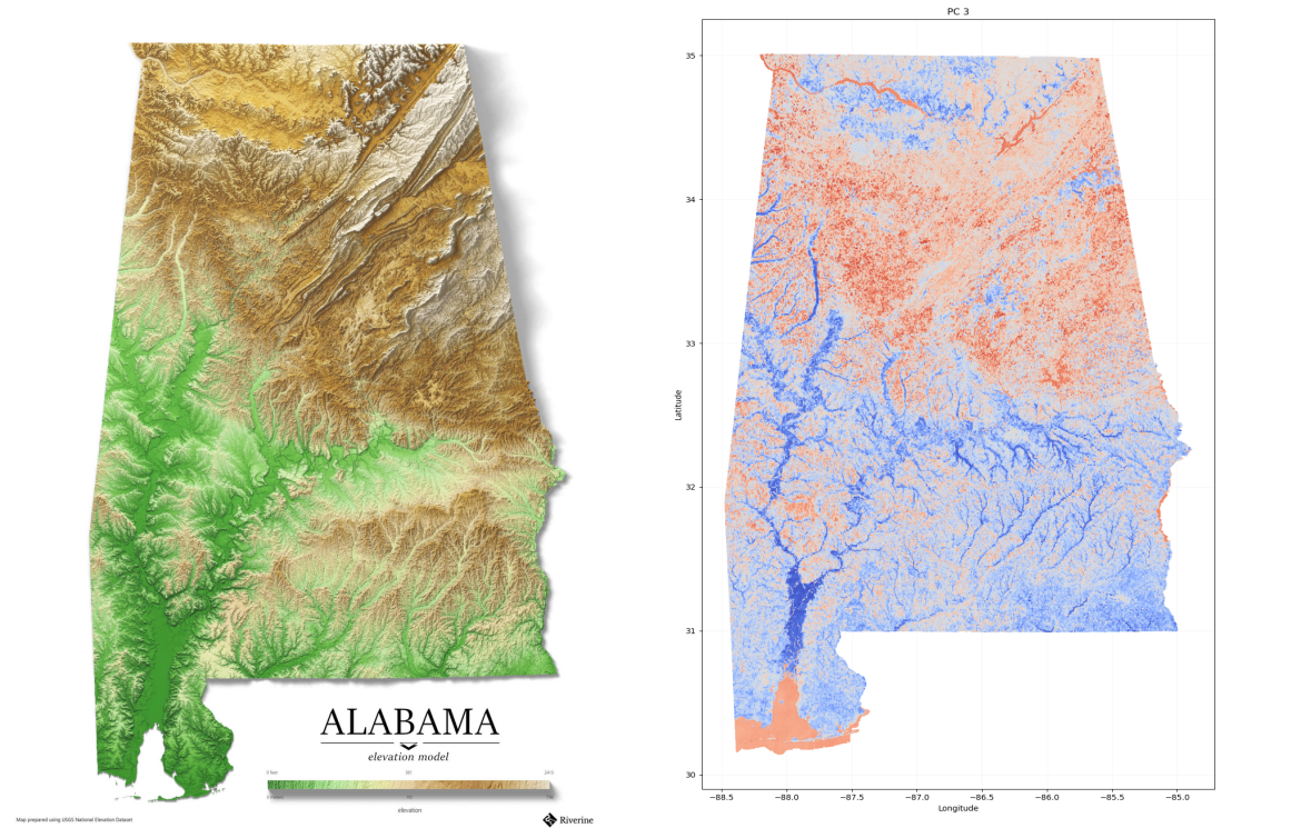
In order to investigate this further, I performed PCA on the 2 millions 64-dim tile embeddings and plotted the first 9 components. We can see the occurence of all sorts of larger scale spatial patterns, and that PC1 and PC3 appear to line up very well with our strange search results! Incidently these explain 20% and 11% of the variance in the full embedding dataset.
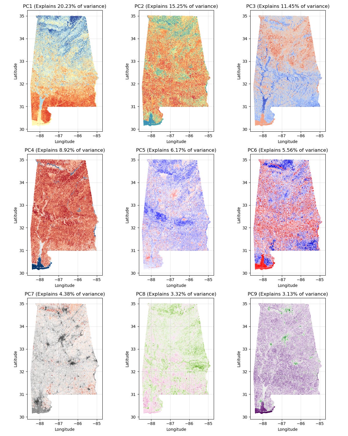
So why might these larger-scale patterns appear? Is there some inherent physical signal driving them? Although I doubt that the embeddings are so well-attuned to the signals from South-Eastern forests that a whopping 20-30% of the variance in them can be attributed to them, we can image since elevation was one of the learning targets, it could somehow distort the latent space:
While this doesn’t appear to be a perfect match, and it’s highly likely that vegetation characteristics would change with elevation, one has to wonder whether they change sufficiently across this territory to warrant this much variance in the embeddings. Should forest in the south of Alabama really be almost semantically closer to wetlands, than forest in the north?
Conclusion
I’d like to commend the Deepmind + Google team for releasing these. These are the first 10m/pixel level embeddings that have been made available to the public, and they are very unique! I’ve had quite a lot of luck searching for something in them (suburbs, golf courses, different types of crops) so they clearly contain some useful information. However I think this sort of unexplained large scale variation across the embeddings for things that humans find semantically similar is ultimately an undesirable property. If I wanted to filter my searches by elevation, that would be a very simple thing to do using a DEM! However if that signal is explicitly incorporated in my embeddings, there is no way for me to get rid of it. Embeddings for retrieval should compress what is hard to join later (texture, specific land-use, shape), not what is trivial (elevation, lat/long, other raster datasets).
As we move towards more people releasing embedding datasets, we need to make sure that the public has the necessary tools and intuition to make use of them. It is also a good thing to do to think about what specific properties you might want your embeddings to have, and adjust model training to reflect that.
Finally: we’ll be releasing tools so that people can do investigations like these soon, so stay tuned!
Acknowledgements
Thank you to Zoe Statman-Weil, Isaac Corley and Noah Golmant for listening to my embedding rants, and for helping me develop these ideas!