
50 ways to compare weather pt 2.
Drought conditions in the lead-up to the 2025 L.A. fires

Please consider donating to aid in the relief of the fires that are affecting L.A. Thank you!
“She said, "It grieves me so to see you in such pain
I wish there was something I could do to make you smile again"
I said, "I appreciate that, and would you please explain
About the fifty ways?"
- Paul Simon
Key Takeaways:
PRISM and ERA5-Land show significant differences in drought severity measurements, with ERA5-Land consistently underestimating drought intensity compared to PRISM, particularly during extreme events like the 2024 LA County drought.
New tools like xee enable easier access to geospatial weather data through Google Earth Engine (GEE), allowing researchers to use familiar xarray/dask ecosystems instead of GEE's frankly odd API. I still think GEE is the 8th wonder of the world though!
I demonstrate a practical implementation of the Standardized Precipitation Index (SPI) using gamma distribution modeling, though alternative distributions and pre-calculated indices (like GRIDMET) are available. The notebook containing the code can be found here.
The analysis reveals record-low SPI calculated over a 6 month period (SPI-6) values for LA County in December 2024, coinciding with the Eaton and Palisades fires, highlighting the real-world implications of drought measurement accuracy, with ERA5-Land underestimating the severity of drought relative to PRISM. PRISM reveals that the SPI-6 for L.A County had a median value of -3, or "Exceptionally Dry/Extreme Drought" according to the World Meteorological Organization, representing a once-in-several-centuries rarity under normal conditions.
Previously on Applied Geospatial:
In part 1, we explored the significant differences between PRISM and ERA5-Land precipitation datasets across the US Corn Belt from 2000-2024. The analysis revealed substantial variations between the two datasets, with precipitation differences exceeding 400mm (40%) in some growing seasons. This variability raises important questions about the reliability of weather-based crop yield models, especially in regions without a gold-standard dataset like PRISM.
Introduction:
The devastating Eaton and Palisades fires that swept through Los Angeles County in January 2025 serve as stark reminders of how drought conditions can fuel catastrophic wildfires. Since I started writing this post, the situation has been further exacerbated by the ignition of the Hughes fire. While news coverage has highlighted the role of precipitation deficits in creating tinderbox conditions, quantifying just how severe these drought conditions were requires careful analysis of historical weather data. Building on our previous exploration of precipitation dataset differences in the US Corn Belt, this post examines the drought conditions preceding these fires using two prominent datasets: PRISM and ERA5-Land. Through the lens of the Standardized Precipitation Index (SPI), we'll investigate how these datasets characterize the extreme dry conditions that set the stage for one of LA County's most challenging fire seasons, while showcasing modern tools that make such analysis more accessible than ever.
Accessing Weather Data on Google Earth Engine:
Thanks to new developments such as xee, an xarray extension for Google Earth Engine (GEE), accessing the precipitation data is as easy as 1, 2, 3! Weather/climate scientists and meteorologists will be happy to find that they do not have to deal with GEE’s esoteric API to access data they want, and instead can use the more familiar xarray ecosystem and perform their calculations client-side, provided they are happy to scale this themselves rather than relying on Google’s servers.
For example: pulling the entire PRISM historical record for LA county can be done in just a few lines. I should note that this dataset is loaded lazily, so we’re able to inspect the metadata very quickly, but anything that requires actually instantiating the data in memory may take a little longer!

Which we can then inspect:
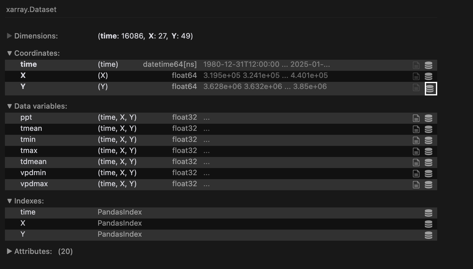
Now that we’ve managed to pull the relevant data (see the ‘ppt’ Data variable in our Dataset), let’s discuss how to calculate and parametrize precipitation using the Standardized Precipitation Index (SPI)
Standardized Precipitation Index (SPI):
The Standardized Precipitation Index (SPI) is an index used to characterize meteorological drought and excess precipitation on a variety of timescales. It is different to ‘standard’ anomaly measure, or z-score, in that it models raw precipitation data as a gamma or a Pearson Type III distribution, rather than as a standard/normal distribution. This is more physically accurate, as precipitation values cannot be negative, and are typically skewed towards smaller amounts. Nonetheless the spirit is similar: quantify observed precipitation within a given timeframe in terms of a standardized deviation from a baseline probability distribution of precipitation.
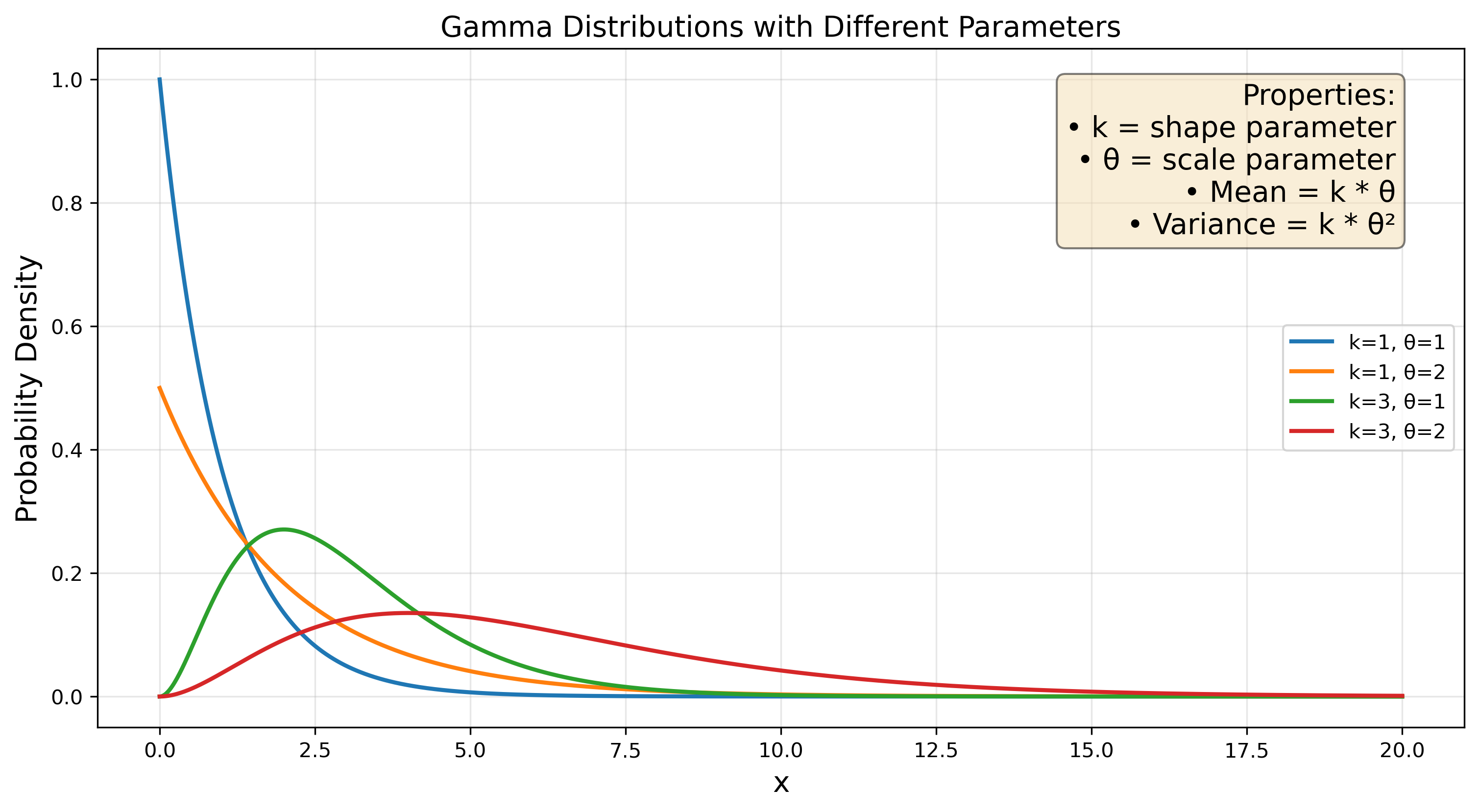
The formula for the gamma distribution is:
where k and theta are the parameters known as ‘shape’ and ‘scale’ respectively.
I’ve plotted some parametrizations here highlighting changes in the key parameters k and theta, or shape and scale. It’s easy to see how they differ from normal distributions in terms of their skew and central tendencies.
Let’s say we are interested in calculating the SPI over a 6 month timeframe (SPI-6) for December in a given location. In essence we are looking to compare the June - December period to a historical baseline for precipitation. These are the steps we need to take:
For our daily dataset, we first resample our dataset to a monthly cadence, then we perform a rolling sum of n_months = 6 across it. To be honest as I’m typing this out I’m realizing we probably could have implemented this rolling sum directly on the data without first resampling.

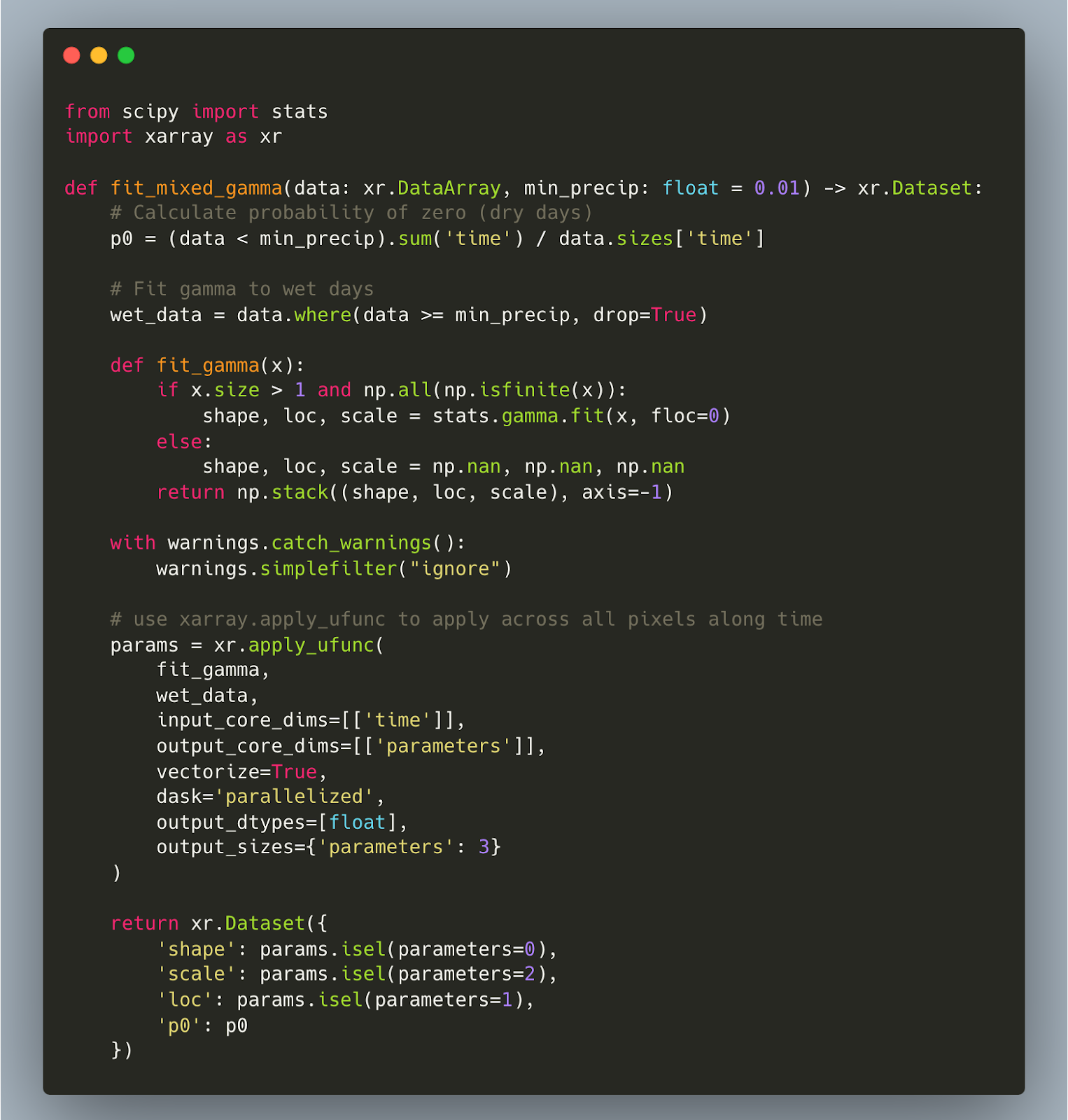
These historical 6-month totals are fitted to a gamma distribution, which captures the characteristic right-skewed nature of precipitation data. A small complication here is that we actually need a separate distribution to characterize the periods for which there is 0 rainfall, because the gamma distribution only deals with positive values. This is called a ‘mixed distribution approach’ where we combine a discrete distribution for "zero" (or trace) precipitation values. We assign probability mass prob_zero to these events and a continuous gamma distribution for non-zero values, which is adjusted by (1-prob_zero) to account for the probability mass already assigned to zeros.
This allows us to calculate the probability of our evaluation precipitation value relative to the baseline mixed distribution. Finally, to broadcast this operation across all the pixels in our dataset, along the time dimension, we use xarray.apply_ufunc. Putting it all together looks like: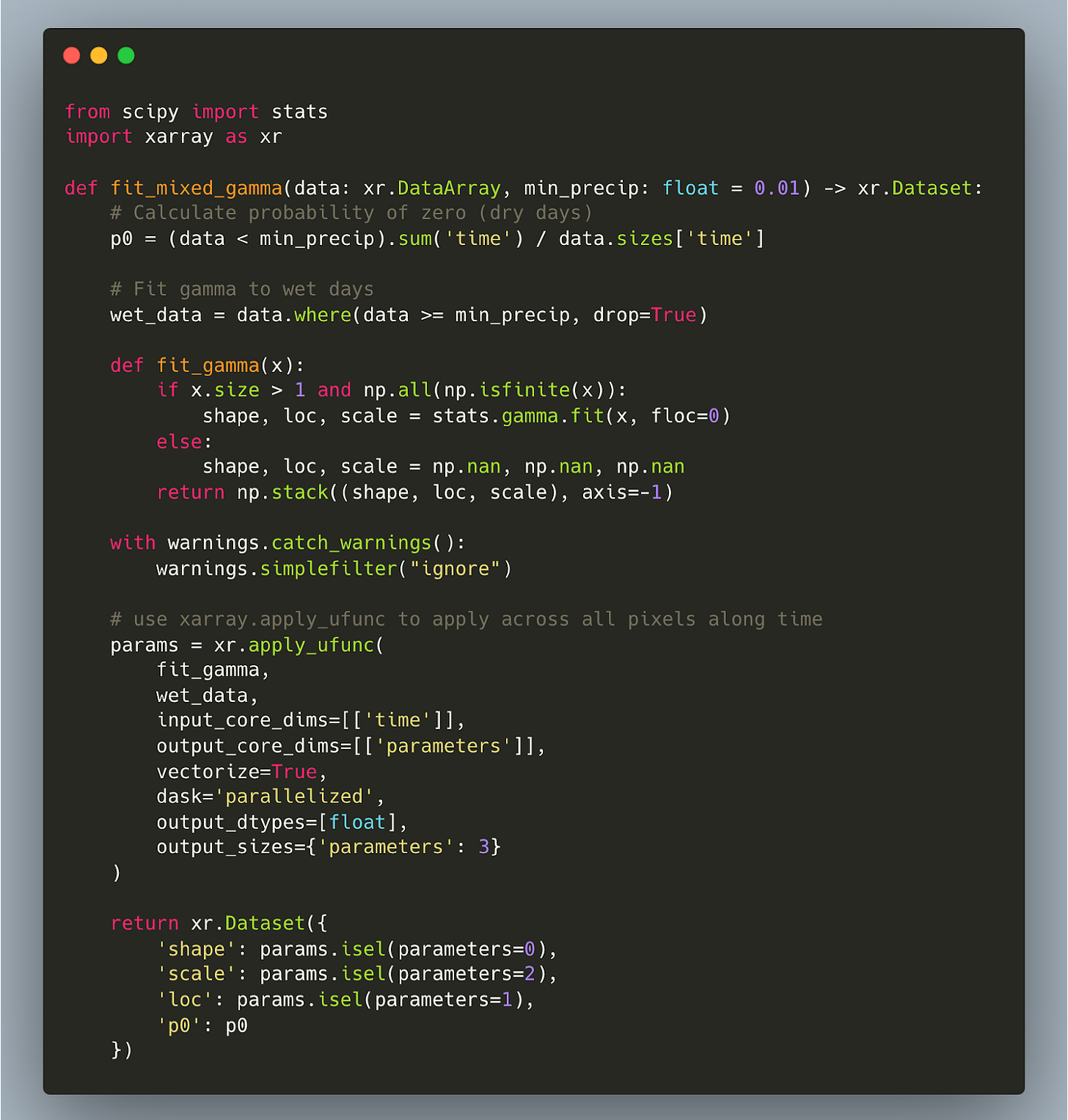
The evaluation period's June-Dec precipitation probability is processed through a gamma-to-normal transformation to obtain its SPI value. We input the probability we calculated into a simple scipy.stats.norm.ppf (Percent Point Function or inverse CDF) which transforms probabilities to standard normal values. Remember, here we need to input the mixed probability distribution, so we’ll need both our gamma probabilities as well as our ‘dry-day’ probabilities:

The SPI gives us a way of expressing the rainfall occurrence for a given period in ‘standard-deviation equivalents’, as if the rainfall were normally distributed. So, when we say an SPI is -1.5, we're saying that rainfall is 1.5 standard deviations below normal, which translates to drier conditions than about 93% of historical observations. This means a -1.5 SPI event should only occur about 7% of the time. The beauty of SPI is that these probabilities work the same way everywhere, whether you're in a desert or rainforest, making it a universal language for describing drought conditions regardless of geography.
That’s pretty much it, for the full implementation, please refer to this colab notebook.
Los Angeles County:
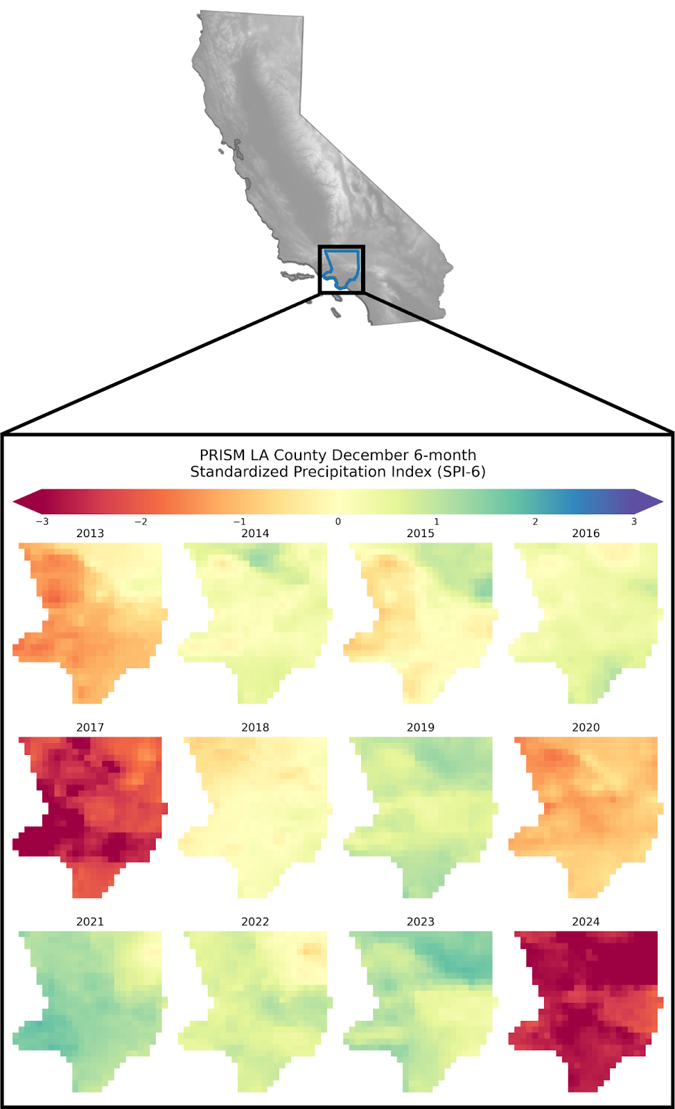
In light of the Eaton and Palisades fires, let’s have a look at what these scores look like for L.A. county in late 2024. Many news articles I’ve come across reference extreme lack of precipitation for that period as one of the causes for the widespread devastation caused by these fires. Since we now know how to calculate the SPI-6, let’s have a look at how bad conditions were in December 2024 relative to the last couple of years using PRISM.
There are actually a number of ways to select a given baseline to construct the gamma distribution for precipitation: we can choose a constant time period, or a changing one. Common SPI lore suggests using a period of at least 30 years, so we’ll use 1981 - 2011 as our constant baseline period. If we examine the December SPI-6 values calculated over L.A. For our evaluation period of 2013 - 2024 we can see that the drought conditions are pretty intense for 2024! We’ll get into the details of exactly how bad these conditions are once we’ve performed our spatial aggregations later in this post.
We can also do the same for ERA5-Land, a much coarser dataset, which extends over a longer time frame (it starts in 1950). We’ll set the baseline range to match the same timescale as PRISM for an accurate comparison (1981 - 2011). Using this dataset we see that the December 2024 period is still the driest in our evaluations.
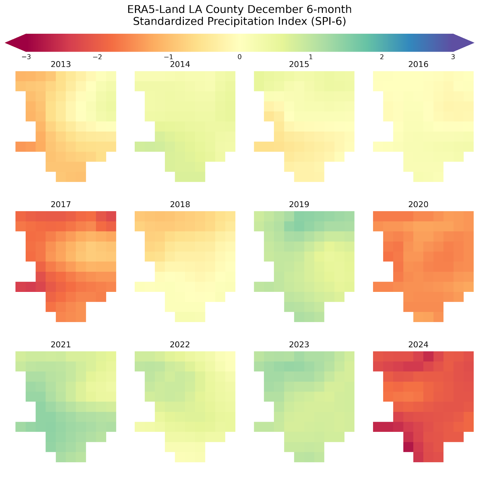
Since apparently we’re in the business of comparing these datasets, let’s aggregate them spatially, and compare the median SPI-6 over L.A. County for all 6-month periods in the last 25 years (not just June - Dec!).

We can see from these time series that ERA5-Land appears to underestimate the magnitude of drought in L.A. County relative to PRISM. As we approach the latter part of 2024, we see that the SPI-6 for L.A. County plummets dramatically, indicating severe drought conditions relative to our baseline. Interestingly though, it appears PRISM SPI-6 continues dropping, while ERA5-Land SPI-6 tapers off a little, resulting in underestimation of the severity of the drought conditions by ERA5-Land. Another way to look at this relationship is via a scatter plot. We can see here that there is better agreement on the SPI-6 value between our datasets for higher values, but the relationship between the two appears to break down a little towards lower SPI-6 values.

Based on our previous understanding of SPI we can now express how bad the conditions were in L.A in December 2024: according to PRISM, the median SPI-6 was close to -3, or the equivalent of -3 standard deviations from historical data if precipitation were normally distributed. This corresponds to a 0.135% chance event based on historical data, underscoring the severity of the conditions!
Conclusion
I tried something a little different for this post, reducing the scale and depth of the study, but attempting to expose more of the practical facets of manipulating geospatial data using tools like xee, GEE and xarray. I’ve also not been as strict with myself on including links/citations, since apparently very few of you are actually clicking on them (that’s right, substack tells me!).
Still we continue to see the pervasive theme from Part 1: these datasets are pretty different: here we see that ERA5-Land appears to underestimate the drought conditions preceding the Eaton and Palisades Fires in L.A. County during December 2024. I should also note that while we used a gamma distribution for precipitation modeling here, there are in fact several candidate distributions one could use to calculate SPI. Another consideration is that the GRIDMET Drought Indices dataset is directly available on GEE, and uses PRISM to derive many drought indices (not just SPI), so one not need go through the convoluted process shown in this post if you are only interested in the indices themselves.
If you enjoyed this post, please consider donating to aid in the relief of the fires that are affecting L.A. Thank you!