
How to Actually Use Embeddings
You can do this too!

TLDR:
I used embeddings to map aquaculture in Alabama.
This map is much better than the one provided by CDL.
When performing this kind of exercise it can be useful to think of first solving the problem at the tile/geometry level, then moving to pixel level if necessary.
You too can use geovibes + existing embedding databases to perform this kind of exercise.
New in geovibes: sampling + classification functionality
New in geovibes: 'detection mode’ : iterate on your classifier outputs.
New in geovibes: add any GEE layer onto your map to help you label.
Two months ago,we released geovibes, a tool that allows users to interact with geospatial embedding databases. The motivation was to allow those who were interested in geospatial embeddings to ‘see for themselves’ rather than be told what embeddings can and can not do by LinkedInfluencers™.
Unfortunately, we released something that falls squarely in the “cool-demo” bucket, and not necessarily the '“actually useful” bucket: yes you could click and find things, but it was still not quite possible to make a map using it. This is an incomplete attempt to rectify this. There is still a lot of work to do!
Opus 4.5 in Claude Code was absolutely instrumental in implementing all of this. I have many thoughts about LLM-based coding/work which I’ll probably explore in a future post, but in my own litmus test of usage, I have not reverted back to OpenAI’s Codex or Cursor since I switched.
Embedding Retrieval
In fair Alabama, where we lay our scene: we start by using geovibes + the Earth Genome provided quantized SSL4EO-pretrained DINO-ViT embeddings which are generated from annual Sentinel-2 composites. We use google maps to search for potential catfish farms to seed our search:
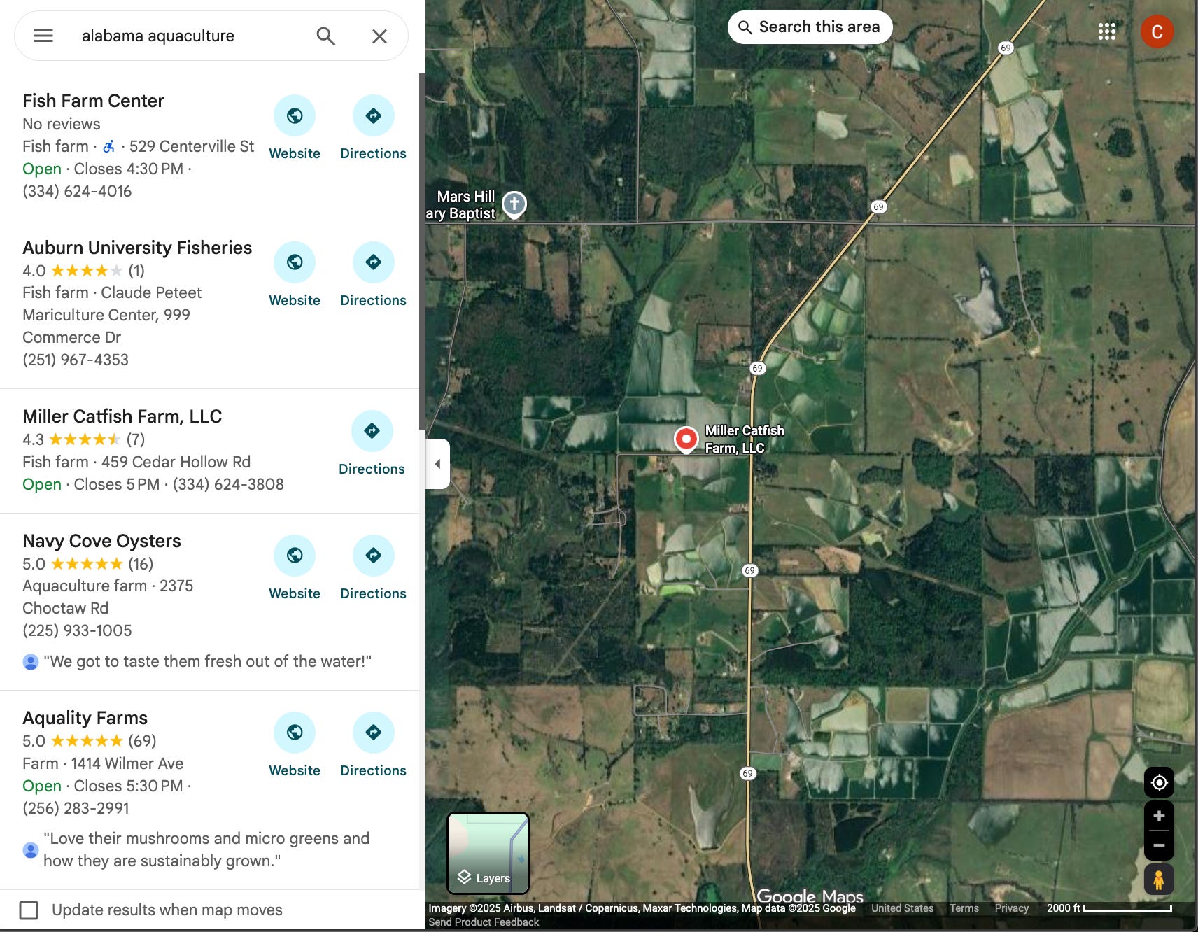
We seed our search with this location in geovibes (still figuring out a better way to do this other than manually), and start searching using our duckdb + faiss index. This results in the following view, where samples all over Alabama are colored by their similarity. In the following video clip I’m:
Seeding the aquaculture search at the Miller Catfish Farm
Opening the tile layer, and sorting the samples by 'most Dissimilar’: aka the samples that are furthest from the initial sample, within the tile layer
Panning around, and collecting those ‘hard negatives’: i.e things that look somewhat similar in the embedding space, that are definitely not aquaculture. You’ll notice many of these tiles are river banks/deltas.
In order to create a classifier: I’ll also label some of the aquaculture positives returned by geovibes. How do I know these are aquaculture? For one, they look like the smooth/green/blue ponds of the Miller Catfish Farm. However, we can also do some research and find out that earthen ponds are the primary method of cultivation for freshwater aquaculture in Alabama1: these are primarily made by digging out a bunch of dirt with a bulldozer and then filling it with water.

Multiple rectangular ponds are laid-out side by side, divided by straight levees. These are typically uniformly sized/shaped, facilitating management and harvesting. This article actually contains a nifty photograph of the harvesting process, which highlights how important the regular shape and proximity to a road is:

Embedding Classification
Now that we have our positives and *some* negatives: we should probably sample some more negatives from our dataset. We’ve implemented two ways to do this in geovibes: you can randomly sample from the duckdb table, or you can do a stratified sample by ESRI/IO landcover map for the year you’re interestsed in. The second method requires a GEE account.
We then filter the sampled negatives if any of them fall within a buffer distance of any of our hard-earned positive samples from geovibes.
Note that if the ‘thing’ you are looking for covers the majority of your area, this will cause some issues for your classifier as you are likely to sample ‘false negatives’. It’s possible that in the future we’ll enable people to use geovibes to post-filter the sampled negatives manually.
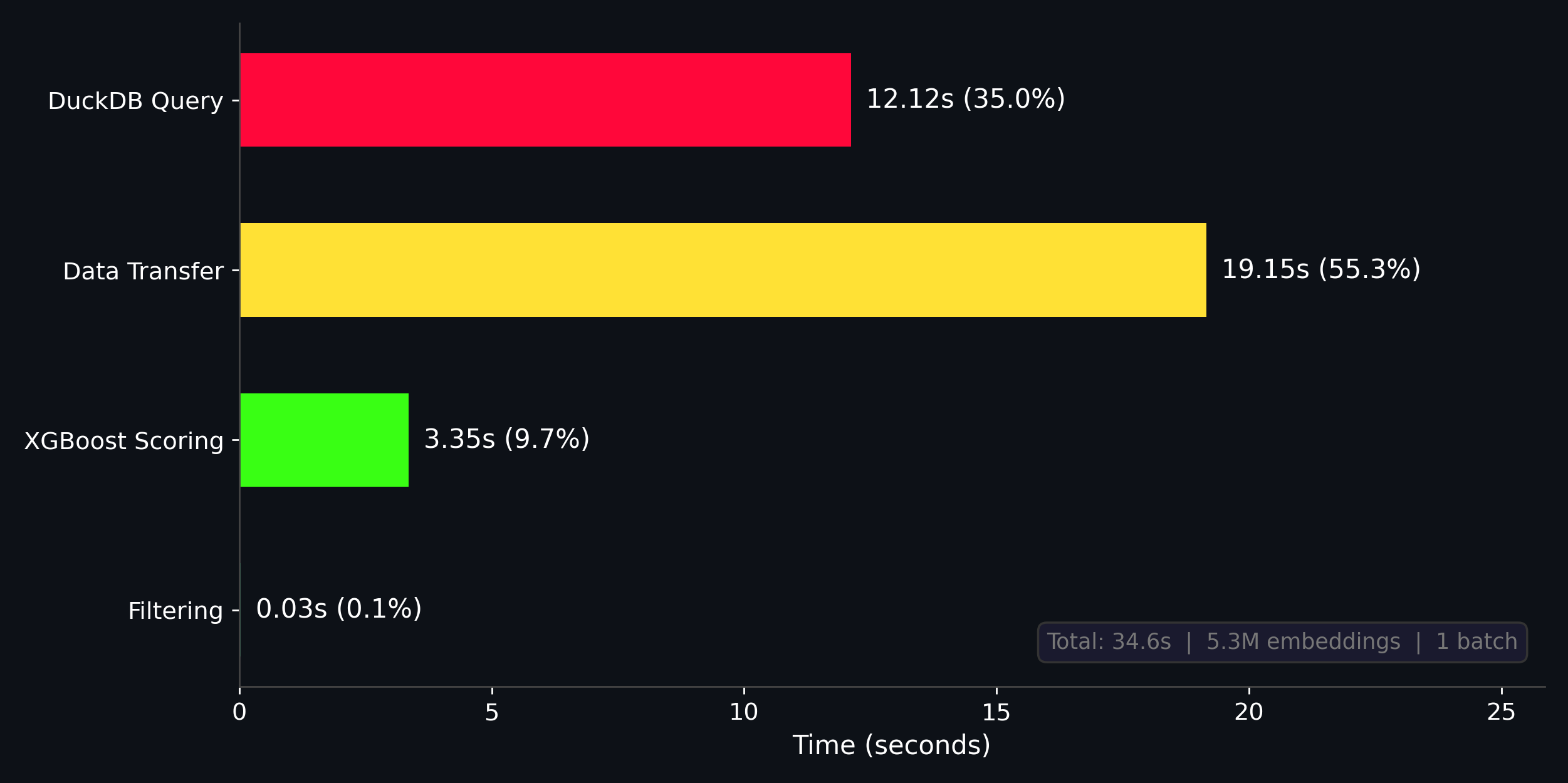
Once we have our geovibes positives, geovibes negatives + sampled negatives, we’re ready to train a classifier! We’ve implemented a pretty simple pipeline with xgboost that:
Trains an xgboost classifier on the dataset
Queries all of the embedding vectors from the duckdb table
Transfers the embedding vectors to a pandas dataframe/numpy array
Uses the trained xgboost model to score the embeddings from the duckdb table
Thresholds the detections by a probability score, and returns both the individual tiles + merged detections for a set probability threshold.
Somehow this process only takes around 40 seconds: our training dataset is quite small (~5000 samples total), but inference is over 5 million 384-dim embeddings! I was quite surprised by this, but then again the 5 million embeddings appear to fit quite comfortably in memory on my 32GB M1 pro, so perhaps this isn’t such a big dataset after all.
Classifier Iteration
We now have a set of detections over Alabama with associated classifier probabilities. We can re-use a lot of the tooling implemented in geovibes to re-label samples, and create a refined dataset for a second round of classification.
In the video below: I show how to load the output of our classification pipeline back into geovibes, I then sort the samples by lowest probability (closest to our threshold of 0.5) and begin labeling again. You’ll notice there are some positives that are on the edge of aquaculture ponds, but also many negatives that occur along the banks of rivers and lakes. In this process, if I am unsure whether a tile is an aquaculture pond or not, I leave it unlabeled.
This process allows us to quickly iterate on our initial embedding classifier using the same framework we did to create our original dataset: quickly viewing and labeling samples of interest. In this case we are using the classifier score/probability as our distance metric rather than a cosine distance.
Interestingly: this re-labeling process which is fairly fast, appears to greatly improve the quality of our classifier. Whereas the initial iteration appeared to struggle with various false postiives such as coastal areas and mining pools, relabeling ~ 300 negatives and positives, which takes around 5 minutes, allows us to improve the classifier a great deal as you can see in the figure below.
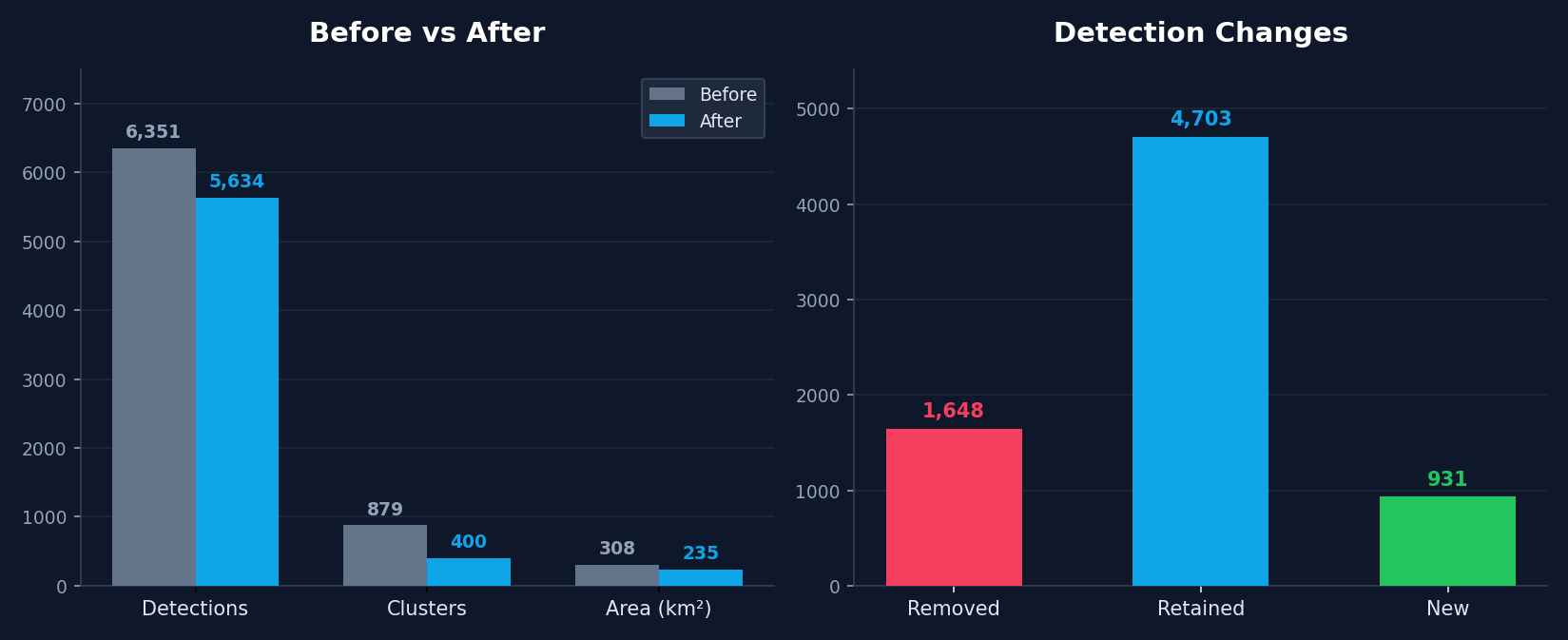
We can have a look at the spatial distribution of the effect of relabeling on our classifier, by looking at where the majority of detections have been:
removed (v0 positive —> v1 negative),
retained (v0 positive —> v1 positive)
gained (v0 negative —> v1 positive)
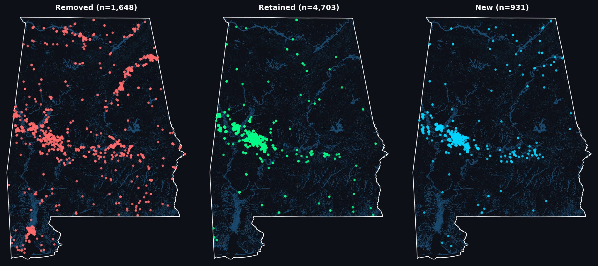
As we can see: many of the removed points are clustered around waterways/water bodies in parts Alabama that most of our labeled aquaculture ponds are not in: to the south near Mobile, as well as North along the Tennessee River, and in the east of the state along the shores of Weiss Lake and the Coosa River. Meanwhile, new detections, in blue, seem to be primarily concentrated in the same region where most of our detections are retained: the Western portion of the Black Belt.
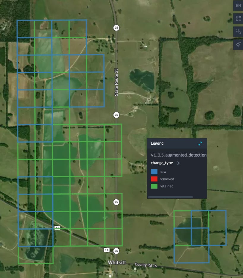
We can take a closer look at where detections have changed to get sense of how the decision boundary of our classifier has shifted: in the Black Belt many of our new detections are at the boundaries/edges of existing aquaculture detections:
Removals in the same area seem to typically be associated with water bodies which have a less regular shape:
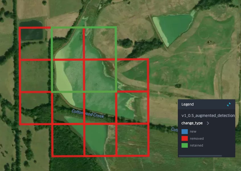
Is this an aquactulture pond? I’m actually not sure (but this is important, more on this below), but it seems unlikely given what we know about levee ponds and aquaculture practices in this region. Another form of removal is found in this area on the edges of a larger set of detections:
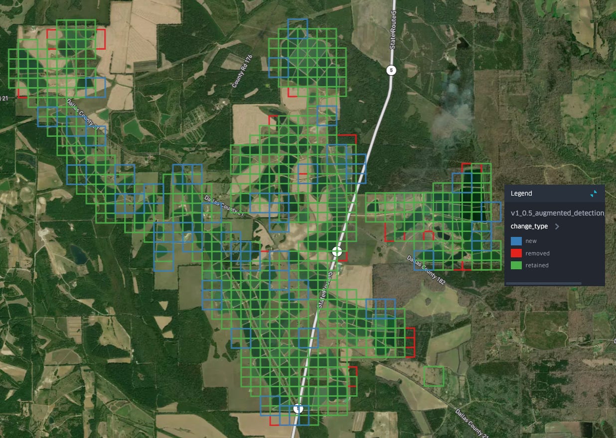
Removals in other areas follow the same pattern: smaller bodies of water, with less regular shapes are now classified as not-aquaculture:
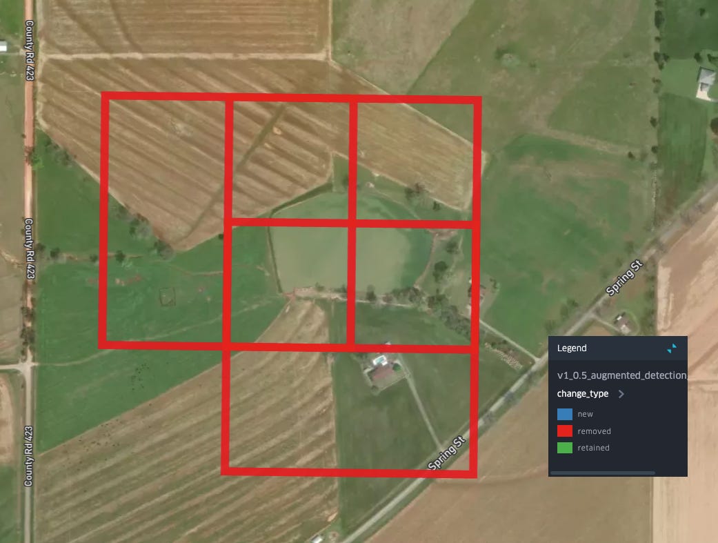
In fact, you can see this reflected in the fact that the total number of clusters detected is reduced by half (~800 to 400) after re-labeling, while the total area is reduced by a lower factor, indicating that the relabeling process has removed many of these smaller detections. After having looked at this set of detections, I’m fairly confident that we have improved the quality of our embedding-based aquaculture classifier!
Tiles to Pixels to Map
People think they want pixel-level maps. For many first passes I believe this is unnecessary and potentially counter-productive. If we had started solving this problem at the pixel level, we would have had to deal with many more rows in our machine learning problem. However, ultimately if we do want a pixel-level map I believe the following workflow is still beneficial: solve the problem at the tile/geometry level first, then within your tiles solve the problem at the pixel level. This greatly reduces the size of the problem.
In this particular case since we know what signal we expect to see over our tiles (water) we can use a land cover map like CDL to simply filter out the non-water pixels. It turns out CDL actually has an ‘aquaculture’ class (in cyan below), but it’s pretty poor and understandably seems to be heavily confused with the ‘open water’ class (dark blue).
In order to produce a map from this:
I manually validated the map, removing a small amount of remaining false positives such as industrial waste ponds and a few remaining coastlines.
I buffered the detections by a half tile.
I selected aquaculture + open water from the latest CDL year over those detections.
That concludes the process of using embeddings to produce a map of aquaculture over Alabama! The final postprocessed geojson can be found here, and the final geotiff at 30m resolution can be found here.
Concluding Thoughts
Looking through these detections, it’s clear to me that the levee-pond style of aquaculture appears to exist in a very geographically constrained area (the Black Belt). This is something that a simple google search would have revealed: a combination of climate, topography and soil type appear to have created ideal conditions for catfish farming. I clumsily georeferenced a soil map with our detections (in red) to highlight this :
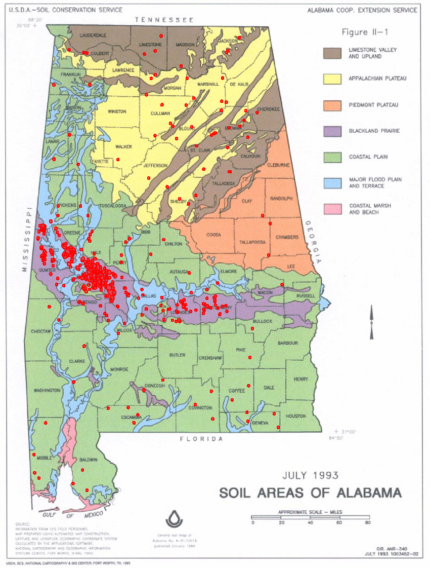
Blackland prairie soil happens to be a dark, heavy, alkaline clay soil, with a very high water retention rate due to the clay content. This means if you dig a hole in it, and fill that hole with water, the water tends to stay! While we chose a data-driven approach to tackle this mapping problem, we could have started from a first-principles approach instead. A little bit of research could have really helped narrow down the area over which we deployed a classifier!
When iterating over the classifier using geovibes, it became obvious to me that the difficulty in these mapping exercises is in the edge cases: sure you can easily map regularly shaped levee ponds, but what about less-regularly shaped ponds, could those be aquaculture as well? How would you determine that/validate? I often found myself using additional information (i.e proximity to industrial parks, or mining areas) to determine if a sample should be labeled as positive or negative.
I think embedding-based workflows face a little bit of a catch-22: yes they are useful, but often a user will require information not contained in the embeddings to perform validation/iterate on their data. If the labels required to do this already exist, then perhaps the problem the user is trying to solve is not an interesting one to solve in the first place. Applications where embeddings will appear to shine initially are ones that can be solved via easy visual verification of (free) medium-resolution imagery: confined animal feeding operations, deforestation/mining, aquaculture. Additionally, there have been demonstrations of the reproduction of existing maps (think USDA’s Cropland Data Layer), while I think these are useful demonstrations of the signal contained in embeddings, it’s not clear to me how one would operationalize these types of models.
https://www.aces.edu/blog/topics/aquaculture/alabama-farm-raised-catfish-industry-highlights/#:~:text=catfish%20from%2055%2C855%20acres%20of,6%20million%20%28figure%201